Oracle 23ai - Models and Embeddings, Part 2

Building a Custom Recommendation Engine

In Part 1 of this series, we explored the powerful new AI capabilities in Oracle 23ai. We saw how we could generate content-based embeddings for our movie dataset, both in a traditional Python environment and then again using a pre-built ONNX model directly inside the database. It was a big success, proving that complex AI tasks are now a native part of the Oracle ecosystem.

However, we also discovered the limits of our simple content-based approach. While it worked for some movies, it often missed the "vibe," recommending movies based on literal keywords rather than their true artistic essence. For 'My Life as a Dog', it recommended other dog movies, completely missing the point.

To create truly compelling recommendations, we need a better model.

In this post, we're going to level up. We will build, train, and deploy our own custom recommendation model from scratch. We'll see how it produces far superior results and how we can integrate it fully into our Oracle 23ai database.

All the source code is available in my GitHub repo.

Key Insights:

• 🚀 Custom ML models in TensorFlow/Pytorch can be loaded into Oracle 23ai as ONNX models, and invoked using SQL.
• 🧠 Embeddings can be learned from structured data to represent any entity, like a customer, a store, or in our case, a movie.
• 🎬 Collaborative Filtering models are typically better at capturing the abstract "vibe" and "essence" of a movie than content-based methods.

A Better Approach: Learning from Human Behavior

Instead of comparing movie descriptions, we will now build a model that learns from the collective wisdom of thousands of users. This technique is called Collaborative Filtering.

The core idea is simple but profound: "You will like what similar people have liked."

This approach completely ignores the movie's title, genres, or tags. It only looks at one thing: the rating patterns in the data. It thinks like this: "Users who gave high ratings to 'The Matrix' also consistently gave high ratings to 'The Thirteenth Floor', even though their text descriptions are different. Therefore, these movies are similar in 'taste'. Since you liked 'The Matrix', I will recommend 'The Thirteenth Floor'."

This is how we capture the magic. A model based on user behavior can uncover latent features like directorial style, pacing, complexity, and that hard-to-define "vibe." It's a much more human-centric way to define similarity, and as we'll see, it produces vastly superior results.

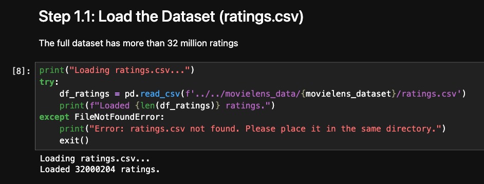
The Dataset

For this Training, we will use the Movielens ratings.csv from the full dataset with 32 million ratings. You can also look at the full Jupyter notebook.

Let's start building the model.

Step 1: Building Our Custom Model in TensorFlow

The content-based model in Part 1 gave us a good baseline, but to capture the true "vibe" of a movie, we need to learn from user behavior. It's time to build our own Collaborative Filtering model from scratch using TensorFlow.

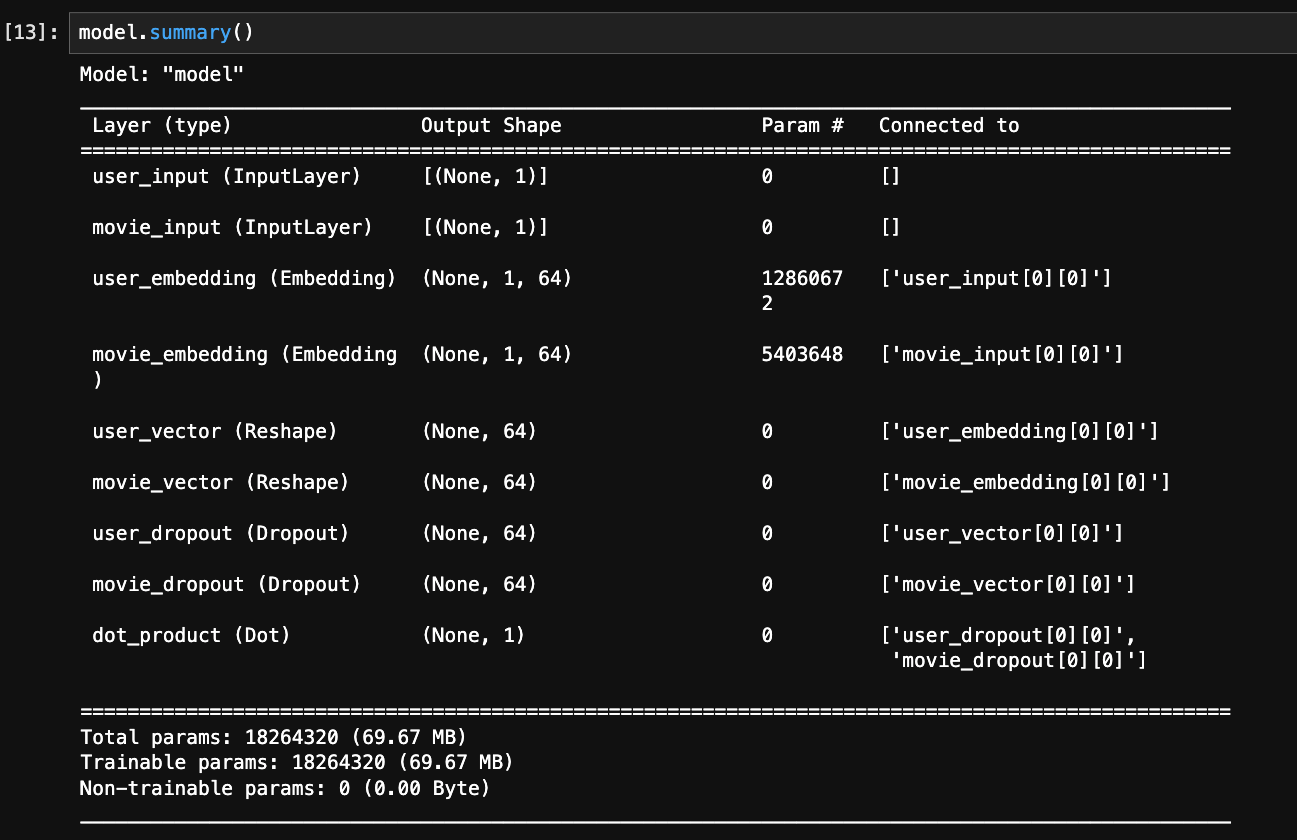
The Model Architecture

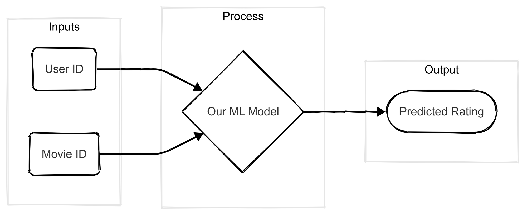
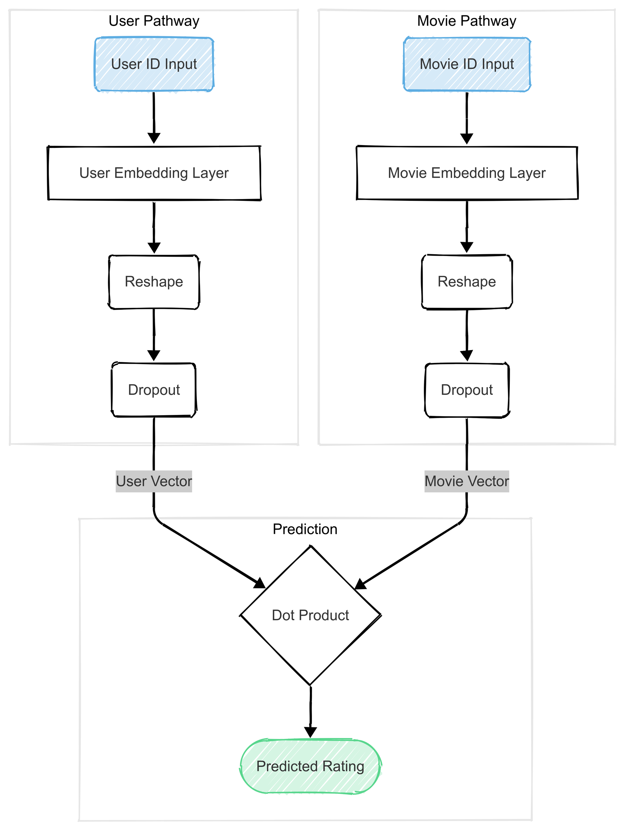
So our goal is to create a model that takes a (userId, movieId) pair and predicts the rating. The technique we'll use is called Matrix Factorization. The architecture is pretty elegant:

1. We have two inputs: one for the user's ID and one for the movie's ID.
2. Each ID is fed into its own Embedding layer. Think of this layer as a large lookup table. The user Embedding layer learns a vector for every single user that represents their unique "taste profile." The movie Embedding layer learns a vector for every movie that represents its "characteristic profile." These vectors are the hidden treasures we're after.
3. We then take the user's vector and the movie's vector and combine them using a Dot product (a bit of Linear Algebra here: We can do that since they are in the same Vectorial space). This produces a single number that is our model's predicted rating.

During training, the model's only goal is to make this predicted rating as close as possible to the user's actual rating.

Note on model type: Since we are trying to predict a number, this is a regression model.

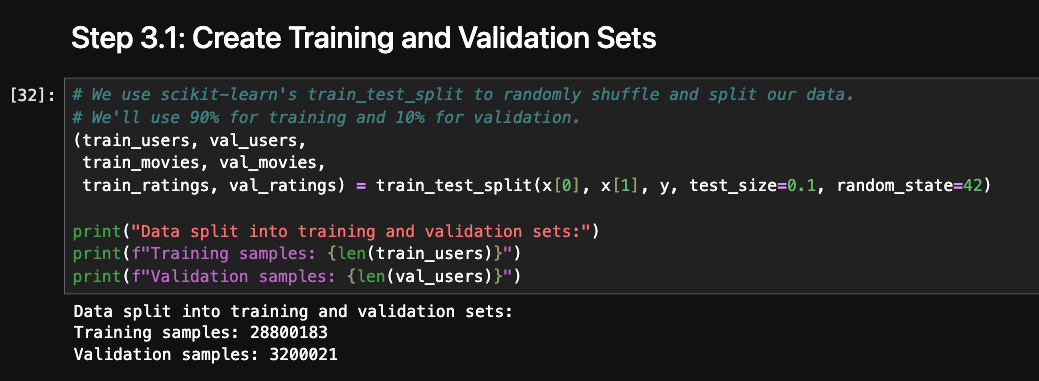
The Importance of a Train Set and a Validation Set

Before we can train, we must split our data. A model can easily "memorize" the data it trains on, leading to a false sense of high accuracy and bad prediction on new data. This is called overfitting.

To check if our model is actually learning general patterns instead of just memorizing, we split our data into two parts:

• Training Set (e.g., 90%): The data the model learns from.
• Validation Set (e.g., 10%): A set of "unseen" data used to check the model's performance after each training pass (called an epoch).

Comparing the model's performance on both sets is the key to building a model that generalizes well.

Training, Overfitting, and a "Textbook" Fix

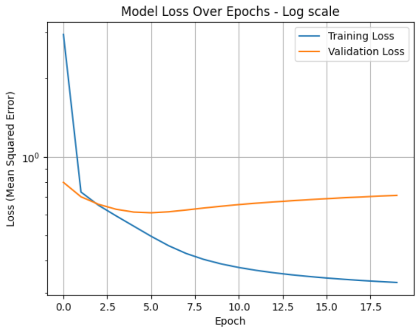
My first attempt at training the model produced a textbook example of overfitting. I let the model train and then plotted its performance (by monitoring the "loss" or error) over time.

Note on Loss: Since it represents how far we are from reality, the lower, the better.

As you can see in the loss curve below, the training loss (blue line) steadily decreases, which is good. However, the validation loss (orange line) decreases for a few epochs and then starts to climb back up. This is the classic sign of overfitting. The model has stopped learning general patterns and is now just memorizing the training data, instead of generalizing for any movies and users.

To fix this, I introduced two powerful techniques:

• Dropout: This regularization technique randomly sets a fraction of the embedding features to zero during each training step. It forces the model to learn more robustly by preventing it from becoming too reliant on any single feature.
• ReduceLROnPlateau: This is a Keras "callback" that monitors the validation loss. If the loss stops improving for a couple of epochs, it automatically reduces the learning rate. This allows the model to take smaller, more careful steps to fine-tune its learned embeddings as it gets closer to a good solution.

After adding these to my model, refining the training hyper-parameters and training again, the result was a much healthier loss curve, showing that our model was now generalizing beautifully.

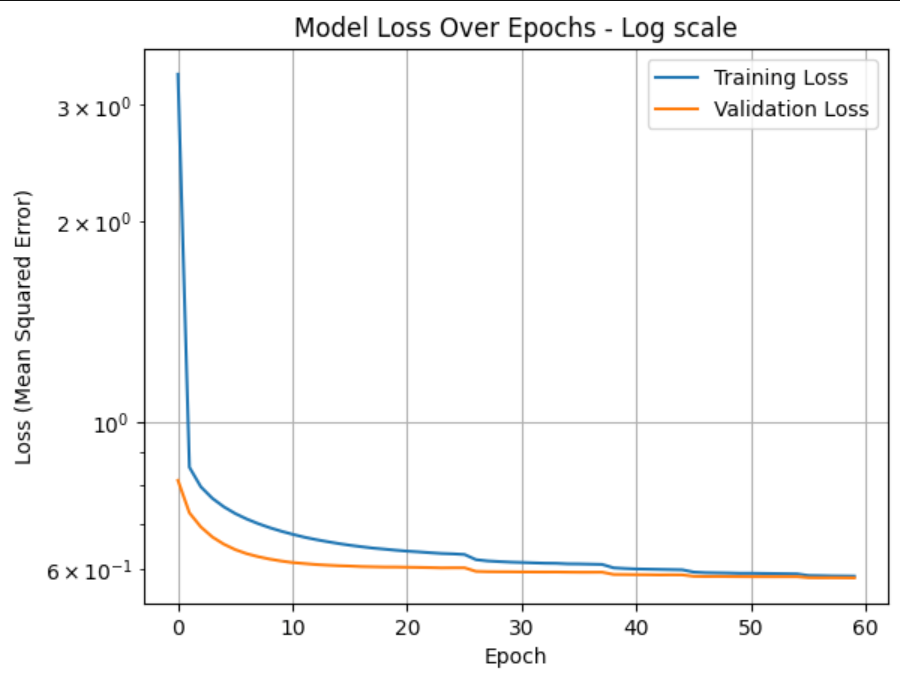
Note how the Validation Loss now always stays near the Training Loss. The reason that it is a bit better (remember: the lower, the better) than the Training Loss is that the regularization (dropout=0.15) is not applied to the Validation set.

With a well-trained and robust model in hand, we are now ready to put it to work.

Step 2: Deploying Our Custom Model in Oracle 23ai

We've successfully built and trained a powerful collaborative filtering model that should understand the "vibe" of movies. But right now, it's just a .keras file on my hard drive. The real power comes from making this model operational. The ultimate goal is to bring this intelligence into the environment where our data lives: the Oracle 23ai database.

This is where the ONNX format becomes essential.

Packaging our Model with ONNX

To get our TensorFlow/Keras model into Oracle, we first need to convert it into the ONNX (Open Neural Network Exchange) format. As we discussed in Part 1, ONNX is the universal translator for machine learning models.

The process involves a Python step that uses the tf2onnx library. A critical step for our two-input model (which takes a userId and a movieId) is to define an input_signature. This explicitly tells the ONNX converter what inputs the model expects. After running the step, we are left with a single, portable cf_recommender.onnx file.

The important parts of the code are:

ONNX_OUTPUT_FILE = os.path.join(MODEL_DIR, "cf_recommender.onnx")

and

# The opset version is important. 13 or 15 are good, stable choices.
print(f"\nConverting model to ONNX with opset 15...")

onnx_model, _ = tf2onnx.convert.from_keras(
    model,
    input_signature=input_signature,
    opset=15
)

and

# Save the ONNX model to a file
onnx.save(onnx_model, ONNX_OUTPUT_FILE)

print(f"SUCCESS: Model successfully converted and saved to:")
print(f"  {ONNX_OUTPUT_FILE}")

Loading the ONNX Model into the Database

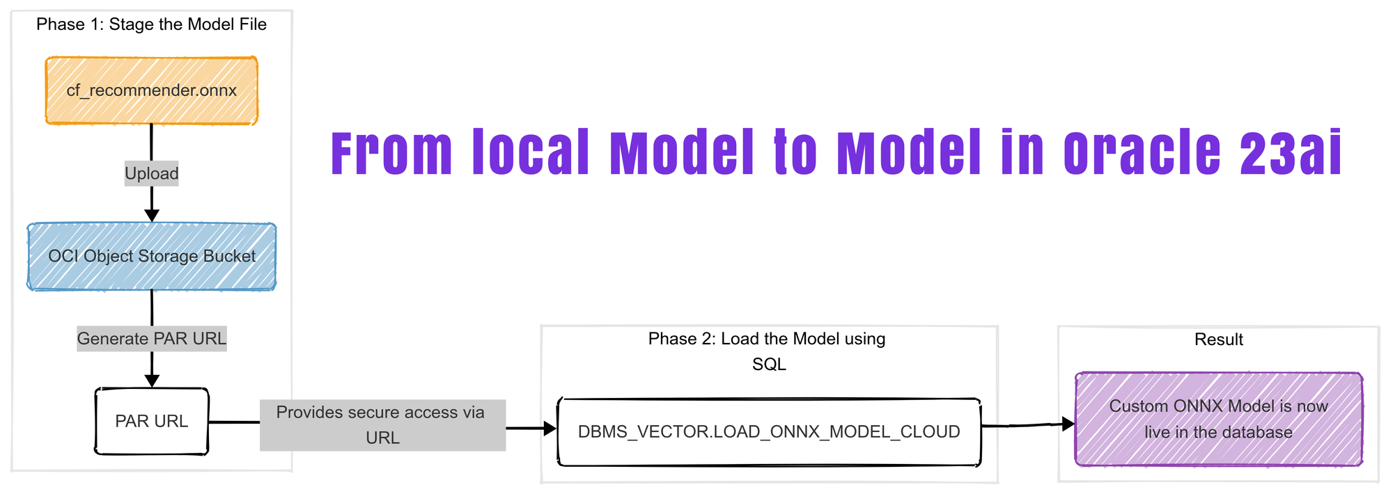
With our cf_recommender.onnx file ready, the next step is to load it into the Oracle 23ai database. The modern, cloud-native approach is to first upload the file to OCI Object Storage.

1. I uploaded cf_recommender.onnx to a bucket in Object Storage.
2. I then created a Pre-Authenticated Request (PAR) for the file. A PAR provides a secure, temporary URL to access the object without needing to configure a full database credential, which is very convenient.

With the PAR URL ready, I used a PL/SQL block in an SQL Worksheet to load the model. The key is the DBMS_VECTOR.LOAD_ONNX_MODEL_CLOUD procedure and the metadata JSON, which acts as a "wiring diagram" for our model. It tells Oracle this is a regression model and maps its internal inputs (user_input, movie_input) to feature names we can use in SQL.

DECLARE
    ONNX_MOD_FILE VARCHAR2(100) := 'cf_recommender.onnx';
    MODNAME       VARCHAR2(500);
    LOCATION_URI  VARCHAR2(500) := 'https://idsvv7k2bdum.objectstorage.us-ashburn-1.oci.customer-oci.com/p/<your PAR URL without the suffix>/b/ONNX-MODELS/o/';
    METADATA_JSON CLOB;
BEGIN
    -- Define a model name for the loaded model
    SELECT UPPER(REGEXP_SUBSTR(ONNX_MOD_FILE, '[^.]+')) INTO MODNAME;
    DBMS_OUTPUT.PUT_LINE('Model will be loaded and saved with name: ' || MODNAME);

    -- --- THIS IS THE CORRECT METADATA FOR YOUR CF MODEL ---
    METADATA_JSON := '
    {
      "function": "regression",
      "input": {
        "user_input": ["USER_IDX"],
        "movie_input": ["MOVIE_IDX"]
      }
    }';

    -- Drop the model if it already exists, to ensure a clean load
    BEGIN
        DBMS_DATA_MINING.DROP_MODEL(MODNAME);
        DBMS_OUTPUT.PUT_LINE('Dropped existing model with the same name.');
    EXCEPTION
        WHEN OTHERS THEN
            NULL; -- Ignore error if model does not exist
    END;

    -- ALTERNATIVELY, TO LOAD FROM CLOUD STORAGE (like your original code)
    -- Ensure your database has the correct network ACLs and credentials set up.
    DBMS_VECTOR.LOAD_ONNX_MODEL_CLOUD(
        model_name     => MODNAME,
        credential     => NULL, 
        uri            => LOCATION_URI || ONNX_MOD_FILE,
        metadata       => JSON(METADATA_JSON)
    );

    DBMS_OUTPUT.PUT_LINE('New model successfully loaded with name: ' || MODNAME);
END;

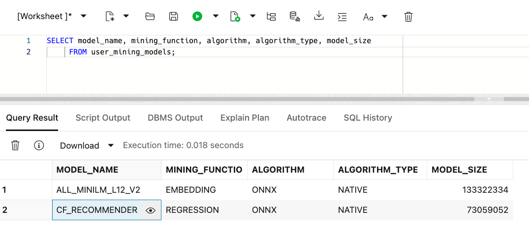
After running the block, the custom model was successfully loaded into my 23ai database, ready to be called.

Let's see the models that are loaded into the database.

Step 3: Making a Live Prediction with SQL

This is the moment everything has been building towards. Our custom TensorFlow model is now a first-class object inside the Oracle database. We can call it directly from a simple SQL query using the PREDICTION function.

The USING clause is where we provide the inputs, mapping our values to the feature names ("USER_IDX", "MOVIE_IDX") we defined in the metadata. Let's see what rating the model predicts for user index 0 (corresponding to user 1) and movie index 0 ('Sense and Sensibility (1995)' is movie 17 mapped to index 0).

SELECT
  PREDICTION(CF_RECOMMENDER USING
    0 AS "USER_IDX", -- or User 1 in movielens 32M full dataset
    0 AS "MOVIE_IDX" -- For movie 17 (Sense and Sensibility (1995),Drama|Romance)
  ) as predicted_rating;

returns 3.9

And just like that, we get our result: 3.9. A very plausible prediction for a movie that I personally rated 4.0! We have successfully built, trained, packaged, deployed, and executed a custom machine learning model, all integrated within the Oracle 23ai ecosystem.

Beyond Regression: A World of In-Database Models

In the previous step, we successfully loaded our custom model by defining its metadata. A key part of that was telling Oracle, "function": "regression", because our model's primary job was to predict a numerical rating.

It's worth noting that this is just one of several model types that Oracle 23ai's ONNX infrastructure supports. By changing that "function" value and providing the correct metadata, you could also deploy models for other common machine learning tasks, such as:

• "classification": To predict a specific category. For example, "Will this customer churn: Yes or No?" or "What is the primary genre of this movie poster: Comedy, Horror, or Drama?".
• "clustering": To group similar items together without pre-existing labels, such as, "Analyze my customer base and group them into five distinct market segments."
• "embedding": As we saw in Part 1, this allows the database to natively use a model to convert raw data like text or images into feature vectors.

This flexibility is incredibly powerful, allowing developers to deploy a wide variety of AI-driven solutions directly into the database, right where their data lives. For our purposes, though, the simple regression function was all we needed to get our model into Oracle. But the story doesn't end there.

The Hidden Treasure: The Learned Embeddings

Making a few rating predictions is a great proof-of-concept, but it isn't the most powerful way to use our new model. The real magic, the hidden treasure, is not the final prediction but the movie and user embeddings that the model learned during training.

Remember, to get good at predicting ratings, the model was forced to create a rich, 64-dimension vector (an embedding) for every single movie. This vector is no longer based on text; it's a numerical representation of the movie's "taste profile" or "vibe," learned from the patterns of thousands of users.

Instead of asking the model for one prediction at a time, we are now going to extract this entire set of learned movie embeddings and load them into our Oracle MOVIES table. Once they are there, we can use the high-speed AI Vector Search capabilities to find the most similar movies.

Loading the "Vibe" Embeddings into Oracle 23ai

The process here will be familiar, combining Python to extract the data from our trained model and SQL to load it into the database.

First, in Python, I wrote a script to load the saved Keras model (collaboration_filter.01.keras.keras), access the movie_embedding layer, and export the final, learned weight matrix. This matrix is our complete set of movie embeddings.

Next, I created a new VECTOR column in my movies table called CF_EMBEDDING to hold these new vectors.

ALTER TABLE movies ADD ( 
   CF_EMBEDDING VECTOR(64, FLOAT32) -- The Collaboration Filter embedding
   );

Finally, I used a Python script with the oracledb driver to execute a bulk UPDATE, loading these new, powerful embeddings into the table, matching them by movieId.

The full script is available here

    print("Connecting to the Oracle Autonomous Database...")
    connection = oracledb.connect(
        user=db_user,
        password=db_password,
        dsn=db_dsn,
        config_dir=wallet_path,  # Tells oracledb where to find tnsnames.ora and other wallet files
        wallet_location=wallet_path,
        wallet_password=wallet_pw
    )
    print("Connection successful.")

    with connection.cursor() as cursor:
        # Define the UPDATE statement
        # sql_insert_statement = "INSERT INTO movies (movieid,  cf_embedding) VALUES (:1, :2)"
        sql_update_statement = "UPDATE MOVIES SET cf_embedding = :1 WHERE movieid = :2"

        # We must tell the driver the type of the first bind variable is VECTOR
        cursor.setinputsizes(oracledb.DB_TYPE_VECTOR, None)

        print("Executing bulk UPDATE with executemany()...")
        # This sends all the updates in an efficient batch
        cursor.executemany(sql_update_statement, data_to_insert, batcherrors=True)

        print(f"Update command sent for {cursor.rowcount} rows.")

        # Commit the transaction
        connection.commit()
        print("Database transaction committed successfully.")

The Payoff: Recommendations that Finally Understand "Vibe"

We've now reached the moment of truth. Our movies table in Oracle 23ai is enriched with two distinct sets of embeddings:

1. Content-Based Embeddings (movie_embedding1): Generated from movie text using a pre-trained language model (done in Part 1).
2. Collaborative Filtering Embeddings (cf_embedding): Learned from user rating patterns using our custom TensorFlow model.

Now we can run the exact same VECTOR_DISTANCE query we've used in Part 1, simply pointing it to our new cf_embedding column, and directly comparing the results.

To find movies that are similar to our 5 movies, I used the same SQL statement as in Part 1, but I refer to CF_EMBEDDING instead of movie_embedding1:

WITH
  -- Step 1: Define the 5 movie titles we want to find recommendations for.
  source_movies AS (
    SELECT 'Apocalypse Now (1979)' AS title UNION ALL
    SELECT 'Inception (2010)' AS title UNION ALL
    SELECT 'Arrival (2016)' AS title UNION ALL
    SELECT 'My Life as a Dog (Mitt liv som hund) (1985)' AS title UNION ALL
    SELECT 'Other Guys, The (2010)' AS title
  ),
  
  -- Step 2: Calculate the cosine distance between our 5 source movies
  -- and every other movie in the main 'movies' table.
  similarity_scores AS (
    SELECT
      s.title AS source_title,
      c.title AS candidate_title,
      -- Use the VECTOR_DISTANCE function on our new in-database embeddings
      VECTOR_DISTANCE(s_emb.CF_EMBEDDING, c.CF_EMBEDDING, COSINE) AS distance
    FROM
      source_movies s
      -- Join to get the embedding for our source movies
      JOIN movies s_emb ON s.title = s_emb.title
      -- Cross join to compare with every candidate movie in the catalog
      CROSS JOIN movies c
    WHERE
      s.title != c.title -- Ensure we don't compare a movie to itself
  ),

  -- Step 3: Rank the results for each source movie independently.
  ranked_similarities AS (
    SELECT
      source_title,
      candidate_title,
      distance,
      -- The ROW_NUMBER() analytic function assigns a rank based on the distance.
      -- PARTITION BY source_title means the ranking (1, 2, 3...) restarts for each source movie.
      ROW_NUMBER() OVER (PARTITION BY source_title ORDER BY distance ASC) as rnk
    FROM
      similarity_scores
  )
-- Step 4: Select only the top 5 recommendations (where rank is 1 through 5) for each movie.
SELECT
  source_title,
  candidate_title,
  distance
FROM
  ranked_similarities
WHERE
  rnk <= 5
ORDER BY
  source_title,
  rnk;

Let's compare our recommendation from Part 1 of this series and Part2 for 'Apocalypse Now (1979)'.

The difference is stunning. The model has completely ignored simple keywords and has instead learned to group movies by their true cinematic essence. The list includes other intense, psychologically complex films from the same era of the 1970s. It found other seminal Vietnam War films (Full Metal Jacket, The Deer Hunter) and masterpieces of gritty character study from the same period (Taxi Driver, Raging Bull).

This is what it means to capture the "vibe." Our custom model, by learning from shared human taste, successfully identified the abstract qualities that make Apocalypse Now a classic.

Other recommendations: You can look at this Jupyter notebook used for training our model to see the top 10 recommendations for 15 movies.

Conclusion of the Series

We started with a simple goal: to explore the new AI features in Oracle 23ai by building a movie recommender. Along the way, we built two complete systems, navigated real-world data loading and model training challenges, and ended with a powerful, custom AI model running directly inside our Oracle database.

I hope this two-part series has shown you a few key things:

• Oracle 23ai is a true AI Platform: It's not just for storing data. It's a powerful environment for both running pre-built models and deploying your own custom AI solutions, keeping your computation and data securely in one place.
• Embeddings Are More Than Just Text: While many think of embeddings for text and images (unstructured data), we demonstrated that you can learn incredibly powerful embeddings from structured, categorical data. This is a huge opportunity for anyone with data in Oracle tables. Think of what you could do by creating embeddings for your own customers, products, stores, or other business entities.
• The Right Model Matters: Choosing the right approach (Content-Based vs. Collaborative Filtering in our case) had a massive impact on our results. Understanding the strengths and weaknesses of different models is a core part of any successful machine learning project.

Finally, my journey wasn't a straight line. I even went down a path of trying to build a complex "Dynamic User Profile" model that ultimately failed, not because of a bug, but because the underlying data signal wasn't strong enough. That "failure" was one of the most important parts of the project as I learned from that. These are the "war stories" that make real-world development so challenging and rewarding.

The gap between the worlds of data science and enterprise data management is closing fast, and Oracle 23ai is building a powerful bridge. I encourage you to start exploring what you can build today.